Jensen Huang used GTC 2026 to reframe how AI infrastructure should be measured. Not FLOPS per dollar, not GPU hours, but tokens per watt. That framing has direct consequences for how you evaluate GPU clouds for inference.
This guide walks through what token factory economics mean in practice, how to calculate the metrics that matter, and which GPU and billing configuration gives you the lowest cost per token on Spheron.
What Is a Token Factory? NVIDIA's Framework for AI Inference ROI
At GTC 2026, Jensen Huang introduced the "token factory" as the right way to think about AI infrastructure investment. The core formula:
Revenue = Tokens per Watt × Available GigawattsThe insight here is that power capacity, not GPU count, is the binding constraint in data centers. A GPU cluster consumes a fixed power budget. Every watt you extract more tokens from directly increases revenue without adding infrastructure cost. For the full picture of why power availability, not GPU count, has become the binding constraint in 2026, see the AI data center power constraints guide.
This reframing matters because raw FLOPS don't map cleanly to business outcomes. A GPU with 2x the FLOPS doesn't produce 2x the inference tokens if it is memory-bandwidth limited. Tokens per watt captures both compute efficiency and memory efficiency in a single number.
"Available Gigawatts" is the scale lever at the infrastructure level. For teams running inference on GPU cloud rather than building out their own data centers, this translates directly to: how many GPU hours can you afford, and how many tokens does each GPU hour produce?
The practical question for anyone running inference on rented GPU compute: given a fixed monthly budget, which GPU model and which billing tier produces the most tokens, and at what cost per million?
The Tokens-per-Watt Metric: How to Calculate It for Your Workload
The calculation is straightforward:
Tokens per Watt = Throughput (tokens/sec) / GPU TDP (watts)Example: H100 SXM5, Llama 3.1 70B, FP8 precision, continuous batching at batch=32:
Throughput: ~2,000 tokens/sec
TDP: 700W
Tokens/Watt: 2,000 / 700 = 2.86
One nuance: actual GPU power draw varies. Memory-bound inference workloads often run below TDP because the GPU is waiting on HBM reads rather than executing tensor operations at full utilization. For sizing purposes, TDP is a reasonable upper bound.
For the full breakdown of how data center power costs translate into per-token electricity bills, including GPU TDP tables and cooling overhead math, see our AI inference power consumption and electricity cost guide.
The companion metric for budget planning is cost per million tokens (CPM):
CPM = ($/hr) / (throughput tok/s × 3,600) × 1,000,000Using the H100 example at Spheron's on-demand rate of $2.90/hr and 2,000 tok/s throughput:
CPM = $2.90 / (2,000 × 3,600) × 1,000,000
    = $2.90 / 7,200,000 × 1,000,000
    = ~$0.40 per million tokens
Three levers move tokens per watt, in rough order of impact:
- Batch size. More concurrent requests per GPU = more tokens per second at the same TDP. The gap between batch=1 and batch=32 is 20-40x throughput at equal power draw.
- Quantization. FP8 versus FP16 on H100 adds 30-40% throughput with no TDP increase. INT4/AWQ can fit a 70B model on a single H100, halving per-token infrastructure cost.
- Framework efficiency. TensorRT-LLM versus a naive PyTorch implementation can double throughput on the same hardware. This is the software lever most teams leave on the table.
GPU Architecture Comparison: Tokens per Watt Across Hopper, Blackwell, and Blackwell Ultra
The table below uses live Spheron pricing fetched on 13 Apr 2026 and throughput estimates for Llama 3.1 70B under continuous batching with FP8 quantization. These are production-realistic numbers with vLLM or TensorRT-LLM at batch=32+, not single-request latency benchmarks.
| GPU | Architecture | HBM | TDP (W) | Est. Throughput Llama 70B (tok/s) | Est. Tokens/Watt | On-Demand $/hr (Spheron) | Spot $/hr (Spheron) |
|---|---|---|---|---|---|---|---|
| A100 SXM4 80GB | Ampere | 80 GB HBM2e | 400 | ~500 | 1.25 | $1.64 | $0.45 |
| H100 SXM5 80GB | Hopper | 80 GB HBM3 | 700 | ~2,000 | 2.86 | $2.90 | $0.80 |
| H200 SXM5 141GB | Hopper | 141 GB HBM3e | 700 | ~2,900 | 4.14 | $4.50 | $1.19 |
| B200 SXM6 192GB | Blackwell | 192 GB HBM3e | 1,000 | ~5,000 | 5.00 | $7.43 | $1.71 |
The H200 wins on tokens per watt for current production hardware despite having the same TDP as the H100. The reason is memory bandwidth: 4.8 TB/s on HBM3e versus 3.35 TB/s on the H100's HBM3. For 70B parameter models, inference is almost entirely memory-bandwidth-limited during the decode phase. More bandwidth means the GPU can read weights faster, which allows larger effective batch sizes at the same power envelope. More concurrent requests at the same wattage = higher tokens per watt.
The B200 adds native FP4 support, which is where the significant efficiency gain comes from at the Blackwell generation. FP4 roughly doubles the theoretical compute throughput versus FP8. The throughput estimate above is conservative for B200, as FP4-optimized deployments can push well above this. The higher TDP (1,000W) limits the per-watt ratio relative to H200 in FP8 comparisons, but at FP4 precision the B200 pulls ahead.
Blackwell Ultra (GB300) is NVIDIA's next iteration within the Blackwell architecture family, a mid-cycle refresh rather than a wholly new generation. Jensen referenced it at GTC 2026 as the continuation of the token factory roadmap. Rubin is a separate, subsequent architecture family expected to follow Blackwell Ultra. Neither GB300 nor Rubin is in broad production deployment on GPU clouds at the time of writing. We won't include speculative benchmark numbers for them here.
See our GPU cloud benchmarks for detailed inference throughput data across providers.
Software Stack Optimizations That Move the Tokens-per-Watt Needle
Hardware generation is the obvious lever, but software often delivers larger gains with zero additional spend. Here are the three worth prioritizing.
TensorRT-LLM and FP8 Quantization
TensorRT-LLM with FP8 on H100 SXM consistently outperforms a vLLM FP16 baseline by 30-40% on throughput for 70B class models. The FP8 Tensor Cores on Hopper (H100 and H200) are native silicon, not emulated, so the precision reduction translates directly into hardware throughput gains.
A100 (Ampere) does not have hardware FP8 support. If you are running FP8 quantization on an A100, it falls back to FP16 compute and you lose the throughput gain. FP8 quantization only pays off on H100 or newer.
For head-to-head numbers across serving frameworks, see vLLM vs TensorRT-LLM vs SGLang benchmarks. For a detailed guide on running SGLang in production with RadixAttention for multi-turn workloads, see the SGLang production deployment guide.
vLLM with Continuous Batching
PagedAttention in vLLM removes KV cache memory fragmentation, which is the main reason naive inference servers fail to scale batch size beyond small values. With PagedAttention, the KV cache can be allocated in non-contiguous pages and reused across requests. The practical effect: you can run batch=64 or higher on an H100 without running out of VRAM.
Higher effective batch size at the same TDP is a direct tokens-per-watt improvement. The delta is large. A single H100 running Llama 3.1 70B FP8 at batch=1 yields roughly 50-80 tokens per second. The same H100 with vLLM continuous batching at batch=32 yields 1,800-2,000+ tokens per second. Same GPU, same power draw, 25-40x more tokens produced per watt.
For a deep dive on KV cache memory management strategies including prefix caching and CPU offloading, see the KV cache optimization guide.
For a full walkthrough of framework setup and serving configuration, see the inference engineering guide.
AWQ and GPTQ for Memory-Constrained Models
Llama 3.1 70B in FP16 requires approximately 140 GB VRAM, which exceeds a single H100 80GB card. The H200 141GB fits the weights, but leaves almost no headroom for the KV cache at meaningful batch sizes. Running it on H100 requires either two GPUs or quantization.
4-bit AWQ brings that memory requirement down to around 35 GB. A single H100 can now run the full 70B model, with VRAM headroom for a substantial KV cache. This halves your per-token infrastructure cost: one GPU instead of two, same output.
The tokens-per-watt impact is significant. You double your throughput per watt by eliminating one GPU from the serving configuration without meaningfully degrading output quality (AWQ is a calibrated quantization method, not brute-force weight rounding).
For a detailed deployment walkthrough, see the AWQ quantization guide.
Choosing the Right GPU Cloud for Token Factory Economics: Spot vs On-Demand vs Reserved
Billing model selection directly affects your cost per token. For a detailed comparison of billing model math across workload types, see GPU billing models compared. For a broader set of cost reduction strategies including auto-shutdown, autoscaling, and multi-cloud arbitrage, see the GPU cost optimization playbook.
Here is the decision framework for inference workloads specifically:
| Workload Type | Recommended Billing | Why |
|---|---|---|
| Development and benchmarking | On-demand | No commitment, short sessions, kill it when done |
| Stable inference traffic (greater than 70% utilization) | Reserved | Best $/hr, predictable cost baseline |
| Burst inference, variable traffic | On-demand | Flexibility over cost optimization |
| Batch inference, latency-tolerant | Spot | 60-75% discount, preemption acceptable |
Spot instances are the right call for batch inference specifically because the workload is stateless and restartable. A preempted batch inference job resumes from its last checkpoint. The user never sees the interruption because there is no user-facing latency requirement. On spot, you take the same GPU at 60-75% lower cost. For a breakdown of Spheron's spot, dedicated, and cluster instance types, see the instance types documentation.
Reserved pricing makes sense only when you are running a GPU at high utilization continuously. The breakeven math: if your on-demand rate is $2.90/hr and reserved saves 30%, you need to use the GPU more than 70% of the time to come out ahead versus on-demand. Most inference workloads have enough traffic variability that reserved overshoots.
On-demand with per-second billing (Spheron bills per second) is the right starting point for any new inference workload. You validate performance and utilization before committing to any contract. For a full breakdown of credits, auto top-up, and team discounts, see the billing documentation. For GPU tier selection and strategies for reducing idle spend, see the cost optimization guide.
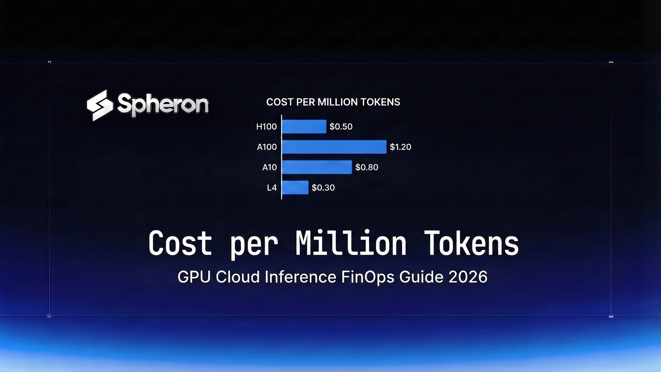
Real-World Token Factory Benchmarks: Cost per Million Tokens on Spheron
This is the number that actually matters for inference FinOps. CPM lets you compare GPU configurations on a single axis regardless of price tier.
Table 1: On-Demand CPM by GPU on Spheron (Llama 3.1 70B)
| GPU | $/hr (on-demand) | Throughput (tok/s) | CPM ($) | Best For |
|---|---|---|---|---|
| A100 SXM4 80GB | $1.64 | ~500 | ~$0.91 | Budget inference, models under 34B, batch jobs |
| H100 SXM5 80GB | $2.90 | ~2,000 | ~$0.40 | Production 70B serving, price-performance sweet spot |
| H200 SXM5 141GB | $4.50 | ~2,900 | ~$0.43 | Memory-bound 70B+ models, high concurrency |
| B200 SXM6 192GB | $7.43 | ~5,000 | ~$0.41 | Maximum throughput, 100B+ models, FP4 workloads |
The H100 lands at the best on-demand CPM for 70B inference. The H200 costs more per hour but delivers proportionally more throughput, keeping its CPM competitive. For teams running 70B models at scale, either H100 or H200 on-demand is a defensible choice depending on whether you hit memory limits with H100.
Table 2: Spot CPM by GPU on Spheron
| GPU | $/hr (spot) | Throughput (tok/s) | Spot CPM ($) | Savings vs On-Demand |
|---|---|---|---|---|
| A100 SXM4 80GB | $0.45 | ~500 | ~$0.25 | 73% |
| H100 SXM5 80GB | $0.80 | ~2,000 | ~$0.11 | 73% |
| H200 SXM5 141GB | $1.19 | ~2,900 | ~$0.11 | 74% |
| B200 SXM6 192GB | $1.71 | ~5,000 | ~$0.10 | 76% |
Spot pricing collapses the CPM. H100 and H200 at spot reach $0.11/M tokens, which is below most managed inference API pricing for open-source models. If your inference workload tolerates occasional preemption, spot is the correct default.
Table 3: Spheron vs Hyperscaler H100 On-Demand
| Provider | H100 On-Demand $/hr | CPM at 2,000 tok/s | vs Spheron |
|---|---|---|---|
| Spheron | $2.90 | ~$0.40 | baseline |
| AWS (p4d equivalent) | ~$4.00 | ~$0.56 | +38% |
| GCP (A3) | ~$3.80 | ~$0.53 | +31% |
| Azure (ND H100) | ~$3.70 | ~$0.51 | +28% |
The hyperscaler premium on H100 is 28-38% above Spheron on-demand. On spot, Spheron reaches $0.11/M tokens versus hyperscaler on-demand at $0.51-0.56/M, a 78-80% cost reduction for workloads that can use spot.
Note: AWS, GCP, and Azure prices in Table 3 are approximate market rates based on publicly listed on-demand pricing and vary by region, commitment tier, and contract terms.
Pricing fluctuates based on GPU availability. The prices above are based on 13 Apr 2026 and may have changed. Check current GPU pricing for live rates.
Scaling a Token Factory: From Single GPU to Multi-Node
Most inference workloads should start on a single GPU and scale only when necessary. The overhead of multi-GPU coordination is real and eats into the per-watt efficiency gain you see on paper.
Single-GPU token factory. One H100 or H200 with vLLM and FP8 quantization handles Llama 3.1 70B at production throughput for most teams below 1 billion tokens per day. Optimize the software stack before adding GPUs.
Multi-GPU within a node. Tensor parallelism lets you split a single model across 2, 4, or 8 GPUs on the same host. This is necessary for models that don't fit in a single GPU's VRAM in the precision you need, or for workloads where a single GPU cannot saturate your latency SLA. NVLink on SXM GPUs keeps the inter-GPU bandwidth high enough that tensor parallelism scales well up to 8 GPUs per node. For H100 8-GPU nodes, TP=8 is the right configuration for 70B FP16 and TP=4 for 70B FP8. For cluster instance specs including NVLink and InfiniBand configurations on Spheron, see the instance types documentation.
Multi-node inference. For models in the 405B+ parameter class, you need multiple hosts. Cross-node communication overhead is significantly higher than within-node NVLink. For a detailed walkthrough of the networking and configuration requirements, see multi-node GPU training without InfiniBand.
Prefill-decode disaggregation. For high-traffic inference at large context lengths, splitting prefill and decode onto separate GPU pools can improve throughput 60-75% over colocated serving. Prefill is compute-intensive; decode is memory-bandwidth-intensive. Routing each phase to hardware suited for it means neither pool has to compromise. See the prefill-decode disaggregation guide for implementation details.
Spheron offers on-demand multi-GPU instances for scale-out configurations without requiring long-term contracts. For programmatic deployment and cluster management, see the API reference.
Where to Start
Token factory economics push toward a clear default configuration for most inference teams:
For latency-sensitive serving of 70B models, start with one or two H100 SXM5s on on-demand, run FP8 with TensorRT-LLM or vLLM continuous batching, and measure your actual CPM before adding more hardware. H200 is worth the step-up cost if you are hitting memory limits or running at high concurrency where its bandwidth advantage materializes.
For batch inference, start with spot H100 or H200. At $0.11/M tokens, the cost case is closed. The only setup cost is adding checkpoint and retry logic, which is a one-time implementation.
The token factory formula works whether you are a startup running one GPU or a team managing hundreds. Every dollar you remove from the denominator (GPU cost) or every token you add to the numerator (throughput) improves your position. Software optimizations and billing model selection move both.
Token factory economics come down to how much compute cost you can eliminate per token generated. Spheron's GPU inventory, H100, H200, and A100, with spot pricing up to 75% below on-demand rates gives you the lowest cost-per-token baseline to build on.
Check H100 availability → | H200 GPU pricing → | View all GPU pricing →
Frequently Asked Questions
A token factory is NVIDIA's framework for thinking about AI inference infrastructure as a revenue-generating unit. The core formula is: Revenue = Tokens per Watt x Available Gigawatts. The GPU cloud that produces the most tokens per unit of power at the lowest cost wins on margins.
Tokens per watt = throughput (tokens/second) divided by GPU TDP (watts). For example, an H100 SXM generating 2,000 tokens/sec at 700W TDP yields approximately 2.9 tokens per watt. You can improve this ratio via quantization, batching, and framework tuning.
The NVIDIA H200 SXM5 leads current production options: its higher HBM3e memory bandwidth allows larger batch sizes at the same power envelope compared to the H100, improving tokens-per-watt by roughly 40-45% on Llama 70B class models. The B200 improves further with FP4 support but at a higher price point.
Spot instances can reduce your compute cost by 60-75% versus on-demand. In token factory terms, lower $/hr directly improves your cost per million tokens (CPM), widening margins without any change to hardware efficiency. The tradeoff is preemption risk, which matters less for stateless inference workloads.
For GPU-intensive inference workloads, Spheron's on-demand H100 pricing typically runs 30-45% below AWS p4d equivalents and 25-40% below GCP A3 instances. Spot pricing on Spheron can be 70-80% below hyperscaler on-demand rates.