At 128K tokens, a 7B transformer's KV cache already exceeds its model weights. At 512K tokens, you need multi-GPU just to hold the cache. This is not a model quality problem; it is a scaling problem, and model size is not the bottleneck anymore.
Two families of architectures have emerged to address this. Linear-attention models (xLSTM, RWKV-7) compress all context into a fixed-size state, achieving O(N) scaling but losing recall past 32K-64K tokens. Full transformers keep exact recall but pay O(N²) in both compute and memory. For background on these tradeoffs, see the xLSTM and RWKV-7 GPU deployment guide and the Mamba-3 SSM deployment guide.
Log-linear attention sits in the middle: O(N log N) scaling via a hierarchical state that grows slowly but retains position-specific recall across the full context window. The architecture is genuinely different from both SSMs and transformers, and it changes which GPU you need for million-token-context workloads.
Why Quadratic Attention Breaks at Long Context and Where Linear Attention Falls Short
The KV cache problem is simple arithmetic. For a 7B transformer at BF16 with 32 layers, 8 KV heads, and 128 head dim, the KV cache memory at sequence length S and batch size B is:
kv_cache_gb = 2 × 32 × 8 × 128 × S × B × 2 bytes / 1e9At 128K tokens, batch size 4: approximately 69 GB. That is on top of ~15 GB for model weights, totaling ~84 GB, which exceeds an H100's 80 GB HBM. At 512K tokens, single request: ~69 GB of KV cache alone. At 1M tokens: ~137 GB.
The prefill compute grows quadratically: double the context, quadruple the attention FLOPs. At 1M tokens on a 70B model, the attention step alone runs into hundreds of petaFLOPs per forward pass.
Linear-attention models solve the memory problem but introduce a recall problem. xLSTM and RWKV-7 compress the sequence into a fixed-size matrix state. The state does not grow with context, so VRAM stays constant regardless of whether you process 4K or 4M tokens. The problem is precision: the fixed state is lossy. Information from early tokens gets mixed, averaged, or forgotten as the model processes more tokens. In practice, needle-in-a-haystack retrieval accuracy on xLSTM and RWKV-7 drops meaningfully past 32K-64K tokens because the state has overwritten earlier information.
The SubQ 1M-Preview guide covers what fully subquadratic architectures look like when they grow linearly rather than quadratically. Log-linear attention is a different point in that design space: it deliberately accepts O(N log N) growth to preserve position-specific recall that fixed-state models lose.
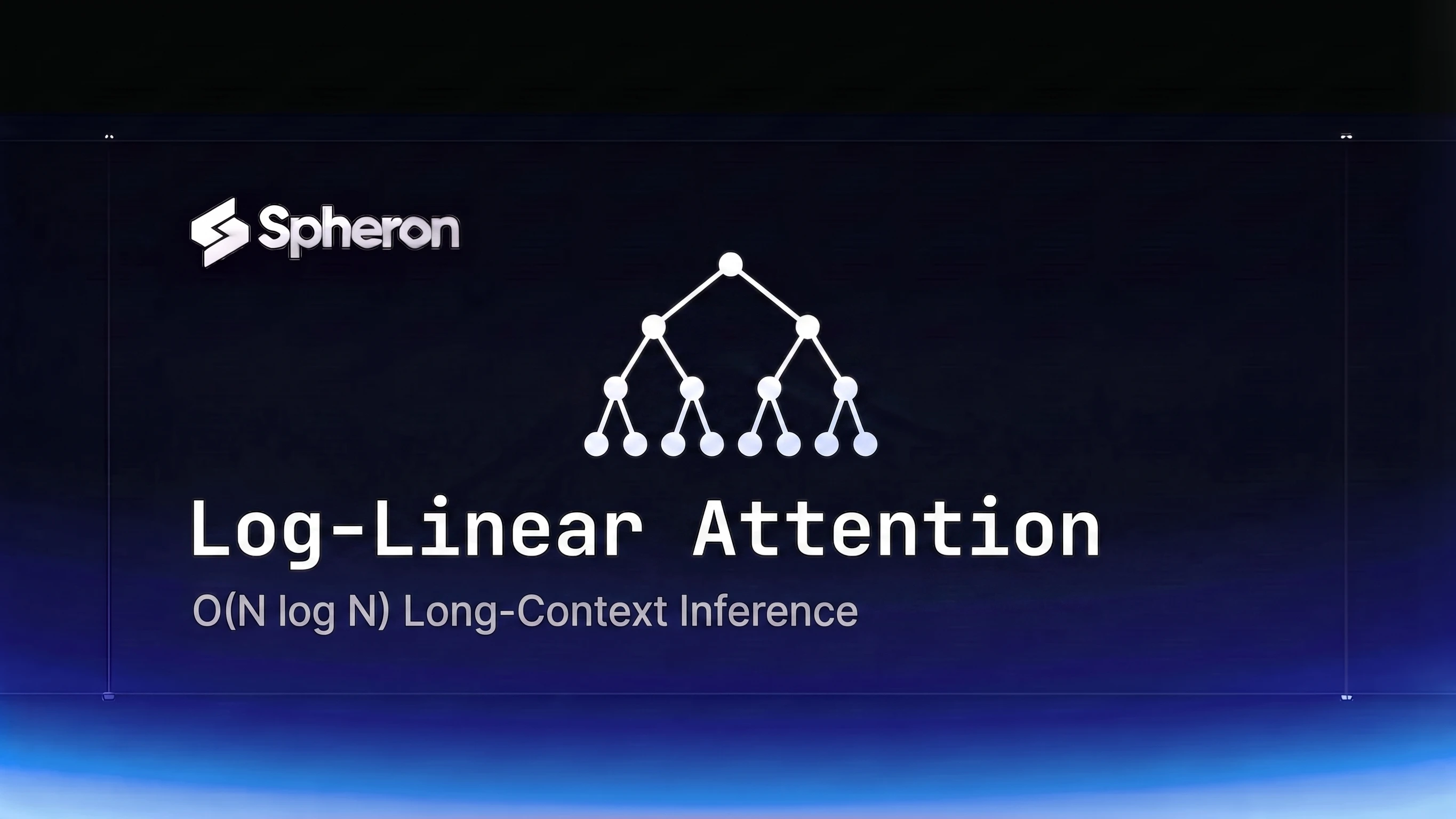
How Log-Linear Attention Works: Hierarchical State and O(N log N)
The core idea is a tree-structured state rather than a flat compressed state.
In a linear-attention model, each new token updates a single state matrix. All prior context is crammed into that matrix. The state has fixed capacity, so old information gets displaced. By token 64K, whatever the model processed at token 1K is largely gone.
Log-linear attention instead maintains a hierarchy: think of it like a Fenwick tree (binary indexed tree) or a segment tree over the sequence. Each level of the hierarchy summarizes a span of tokens that doubles at each level up. Level 0 holds individual recent tokens. Level 1 summarizes pairs. Level 2 summarizes groups of four. Level log(N) summarizes the entire prefix.
When processing a new token at position N, the model queries O(log N) levels of the hierarchy. Near-recent tokens are retrieved with fine granularity (level 0 or 1). Distant tokens are retrieved via coarser level summaries. The total state size at position N is O(log N): the number of hidden states in the hierarchy grows logarithmically, and each state has fixed size. This is far smaller than the O(N) KV cache of a full transformer, and unlike fixed-state SSMs, each level remains individually addressable.
The state-update cost per token is O(log N) operations, which gives O(N log N) total training cost. At inference time, each new token requires reading O(log N) state levels and writing one new entry at the appropriate levels. This is more expensive than an SSM's O(1) state read but far cheaper than a transformer's O(N) attention over the full context.
The Tree Attention mechanism described in the Ring and Tree Attention sequence parallelism guide uses a related logarithmic communication topology across GPUs. The mathematical structure is the same: log(N) rounds of merging rather than N rounds. Log-linear attention applies this idea to the attention mechanism itself rather than to multi-GPU communication.
The state at a given context length differs across architecture families:
| Architecture | State size at 1M tokens | State type |
|---|---|---|
| Full transformer | ~137 GB KV cache (7B BF16) | Explicit per-token KV pairs |
| Log-linear attention | ~2 GB (directional) | Hierarchical tree structure |
| Linear attention / xLSTM / RWKV-7 | ~2-4 GB (fixed) | Fixed-size recurrent matrix |
| SSM / Mamba-3 | ~2-4 GB (fixed) | Fixed-size recurrent state |
These are directional estimates. Actual figures depend on the specific architecture, number of layers, head dimensions, and precision format used.
Log-Linear vs Linear Attention vs SSMs vs Sparse Attention: Decision Matrix
The five main architecture families each occupy a different position in the scaling-quality tradeoff:
| Architecture | Complexity | VRAM at 1M tokens (7B BF16, directional) | Recall at 256K+ | Framework support (Jun 2026) | Best use case |
|---|---|---|---|---|---|
| Full transformer | O(N²) | ~137 GB | Exact | vLLM, SGLang, TGI (native) | Short-to-medium context, maximum quality |
| Log-linear attention | O(N log N) compute, O(log N) memory | ~2 GB | Near-exact | Custom PyTorch / patched vLLM | Long-context tasks requiring position-precise recall |
| Linear / xLSTM / RWKV-7 | O(N) fixed state | ~2-4 GB | Degrades past 32K-64K | Custom runtimes, partial vLLM | Very long context, throughput-first, recall not critical |
| SSM / Mamba-3 | O(N) fixed state | ~2-4 GB | Degrades past 32K-64K | vLLM (supported), SGLang | Long context, compute-bound workloads |
| Sparse / DSA | O(N × K), K fixed | Depends on K | High for top-K relevant | vLLM (DSA backend), SGLang | Long context with learned token selection |
The DeepSeek Sparse Attention guide covers DSA in depth. FlashAttention-4 covers how to make full transformer attention as fast as possible on Blackwell hardware.
Log-linear attention is the right choice when you need both long context and high recall, but full transformer cost at 512K-1M tokens is prohibitive. If recall accuracy at 128K+ is not critical, Mamba-3 or xLSTM are cheaper per token. If you need exact attention quality and can pay the compute cost, full transformers with FlashAttention-4 are better supported in production tooling today.
Inference Characteristics: Memory Footprint, Throughput, and Quality at 256K-1M Context
Memory footprint
The O(log N) state growth means memory planning for log-linear attention differs from both the linear and quadratic cases:
| Context length | Full transformer KV (7B BF16) | Log-linear state (7B BF16, directional) | Linear/SSM state (7B BF16) |
|---|---|---|---|
| 64K | ~9 GB | ~1.7 GB | ~2-4 GB (fixed) |
| 128K | ~18 GB | ~1.8 GB | ~2-4 GB (fixed) |
| 256K | ~35 GB | ~1.9 GB | ~2-4 GB (fixed) |
| 512K | ~69 GB | ~2.0 GB | ~2-4 GB (fixed) |
| 1M | ~137 GB | ~2.2 GB | ~2-4 GB (fixed) |
These state sizes are directional. At 256K tokens, log-linear attention adds only ~1.9 GB to the model's base VRAM (~15 GB for 7B BF16), putting total memory around 17 GB. An H100 SXM5 (80 GB) handles this comfortably with large batching headroom. At 1M tokens, the ~2.2 GB hierarchical state brings total VRAM to ~17 GB, still fitting easily on a single H100. An H200 SXM5 (141 GB) is the better option when high batch concurrency is needed at 512K-1M context for 7B models.
Throughput
Log-linear attention's sequential state-update pass creates a prefill bottleneck that full transformers with FlashAttention-4 do not have. At short contexts (under 32K tokens), log-linear models are slower on prefill than FlashAttention-optimized transformers because the hierarchical state updates are serialized per level. At 256K-1M tokens, the O(N log N) cost beats O(N²) handily.
Directional decode throughput on H200 SXM5 for a 7B log-linear model (single request, one token per step):
| Context length | Approximate decode tokens/sec (H200, directional) |
|---|---|
| 128K | ~85-100 |
| 512K | ~60-75 |
These figures assume each new decode step requires reading O(log N) state levels: roughly 17-20 reads at 512K context. Actual throughput varies by implementation quality and kernel optimization. The sequential nature of the state read limits parallelism compared to a transformer's ability to batch attention across all positions at once.
Recall quality
The key quality differentiator for log-linear attention is needle-in-a-haystack retrieval: finding a specific piece of information buried in a long context.
Fixed-state models (Mamba-3, xLSTM, RWKV-7) perform well on needle retrieval up to 32K-64K tokens. Past that length, the fixed state has been overwritten enough times that early-context information becomes unreliable. In practice, recall accuracy on hard needle-in-a-haystack tests drops to 70-80% at 128K and further at 256K for most fixed-state models.
Log-linear attention retains O(log N) granularity per position. Each position at distance D from the current token is summarized at resolution 1/2^k where 2^k is the nearest power-of-two span containing D. This means positions from 256K tokens ago are summarized in a span-256K bucket, which is coarser than the span-1K bucket covering recent tokens, but still a specific, addressable piece of state. The SubQ guide's discussion of recall framing is the right conceptual reference: full recall quality requires either full attention (O(N²)) or a state that encodes position-specific information at non-trivial resolution.
Log-linear attention targets that middle ground. The xLSTM and RWKV-7 throughput tradeoff section documents exactly where fixed-state recall degrades; log-linear attention's raison d'être is the set of workloads that sit past that boundary.
Current Implementations and How to Serve Them on GPU Cloud
As of June 2026, log-linear attention is primarily a research architecture. Production deployments use one of three approaches:
1. PyTorch reference implementations. Research papers typically release PyTorch reference code on HuggingFace or GitHub. These run single-request inference but lack batching, multi-GPU support, or production serving infrastructure. Good for evaluation; not for production.
2. FastAPI + stateful PyTorch runtime. The production-viable path today is a FastAPI wrapper around the PyTorch forward pass, with the hierarchical state tensor held in GPU memory between turns. This supports stateful multi-turn sessions without replaying the full context on each turn.
3. Patched vLLM builds. Some research teams have published vLLM forks with custom attention backends for log-linear attention. These are model-specific and not merged into mainline vLLM. Check the specific model's HuggingFace model card for serving recommendations.
Here is the FastAPI + stateful state management pattern for a multi-turn log-linear attention server:
from fastapi import FastAPI
from pydantic import BaseModel
import torch
from typing import Optional
import uuid
import threading
import time
from collections import OrderedDict, defaultdict

app = FastAPI()
model = None

MAX_SESSIONS = 50      # evict oldest when limit is reached
SESSION_TTL = 3600     # drop sessions idle for more than 1 hour

class _LRUStateCache:
    """LRU cache capped at MAX_SESSIONS with per-entry TTL to prevent GPU OOM.

    Without eviction, every long-context session holds 1.5-3.5 GB of hierarchical
    state tensors in CUDA memory indefinitely, causing the server to OOM after
    many concurrent sessions. on_evict lets callers clean up other per-session
    state (e.g. the lock in _session_locks below) so it doesn't leak unbounded.
    """
    def __init__(self, max_size: int, ttl: int, on_evict=None):
        self._cache: OrderedDict = OrderedDict()
        self._last_access: dict = {}
        self._max_size = max_size
        self._ttl = ttl
        self._lock = threading.Lock()
        self._on_evict = on_evict

    def get(self, key, default=None):
        with self._lock:
            if key not in self._cache:
                return default
            if time.monotonic() - self._last_access[key] > self._ttl:
                self._evict(key)
                return default
            self._cache.move_to_end(key)
            self._last_access[key] = time.monotonic()
            return self._cache[key]

    def __setitem__(self, key, value):
        with self._lock:
            if key in self._cache:
                self._cache.move_to_end(key)
            else:
                while len(self._cache) >= self._max_size:
                    oldest = next(iter(self._cache))
                    self._evict(oldest)
            self._cache[key] = value
            self._last_access[key] = time.monotonic()

    def _evict(self, key):
        state = self._cache.pop(key, None)
        self._last_access.pop(key, None)
        del state  # release memory immediately; works for plain tensors and hierarchical state (tuples, dicts, etc.)
        if self._on_evict:
            self._on_evict(key)

_session_locks: dict = {}             # session_id -> Lock, serializes read-inference-write per session
_session_lock_refs: dict = defaultdict(int)  # session_id -> number of threads currently checked out
_session_locks_guard = threading.Lock()      # protects the two dicts above

class _SessionLock:
    """Checks out the per-session lock without racing the LRU evictor.

    `with _session_locks[session_id]:` looks like one atomic step but is
    actually two: a defaultdict lookup, then lock.acquire(). The GIL can
    switch threads between them, so a thread could acquire a lock object
    that _evict_session_lock has already popped and released, while a
    second thread gets a brand-new Lock for the same session_id, letting
    both run model.generate() concurrently. Fixing this means the
    lookup-and-checkout has to be one atomic step, and an entry must never
    be removed while any thread still holds a reference to it, whether
    that thread is actively inside the critical section or just waiting on
    lock.acquire(). A refcount tracks that: it's incremented before
    lock.acquire() is even called, and only an entry with a zero refcount
    is eligible for eviction.
    """
    def __init__(self, session_id):
        self._session_id = session_id

    def __enter__(self):
        with _session_locks_guard:
            lock = _session_locks.setdefault(self._session_id, threading.Lock())
            _session_lock_refs[self._session_id] += 1
        try:
            lock.acquire()
        except BaseException:
            with _session_locks_guard:
                _session_lock_refs[self._session_id] -= 1
                if _session_lock_refs[self._session_id] <= 0:
                    _session_locks.pop(self._session_id, None)
                    _session_lock_refs.pop(self._session_id, None)
            raise
        self._lock = lock
        return self

    def __exit__(self, exc_type, exc, tb):
        self._lock.release()
        with _session_locks_guard:
            _session_lock_refs[self._session_id] -= 1
            if _session_lock_refs[self._session_id] <= 0:
                _session_locks.pop(self._session_id, None)
                _session_lock_refs.pop(self._session_id, None)

def _evict_session_lock(session_id):
    # Only drop the lock entry if no thread currently has it checked out.
    # Checkout increments the refcount atomically with the dict lookup (see
    # _SessionLock.__enter__), so this can never remove a lock object out
    # from under a thread that's already holding or waiting on it.
    with _session_locks_guard:
        if _session_lock_refs.get(session_id, 0) == 0:
            _session_locks.pop(session_id, None)
            _session_lock_refs.pop(session_id, None)

states = _LRUStateCache(
    max_size=MAX_SESSIONS,
    ttl=SESSION_TTL,
    on_evict=_evict_session_lock,  # keep lock count bounded, but never while a request is using it
)

class GenerateRequest(BaseModel):
    prompt: str
    session_id: Optional[str] = None
    max_new_tokens: int = 256

@app.on_event("startup")
async def load_model():
    global model
    # Replace with your log-linear attention model loader
    from your_model_package import LogLinearAttentionModel
    model = LogLinearAttentionModel.from_pretrained("your-model-id").cuda().bfloat16()
    model = torch.compile(model, mode="reduce-overhead")

@app.post("/v1/completions")
def generate(req: GenerateRequest):
    session_id = req.session_id or str(uuid.uuid4())
    with _SessionLock(session_id):  # serialize concurrent requests on the same session_id
        prev_state = states.get(session_id)

        inputs = model.tokenizer(req.prompt, return_tensors="pt").to("cuda")

        with torch.inference_mode():
            output, new_state = model.generate(
                **inputs,
                hierarchical_state=prev_state,
                max_new_tokens=req.max_new_tokens,
            )

        states[session_id] = new_state  # LRU cache evicts oldest when MAX_SESSIONS is hit

    text = model.tokenizer.decode(output[0], skip_special_tokens=True)
    return {"session_id": session_id, "text": text}
The key line is hierarchical_state=prev_state: passing the state from the previous turn lets the model continue from where it left off without reprocessing the full conversation history. This is what makes stateful multi-turn efficient for log-linear attention models at long context.
For kernel compilation, torch.compile(model, mode="reduce-overhead") is the correct starting point. For more advanced CUDA graph capture to eliminate Python overhead on repeated calls, see the torch.compile and CUDA Graphs guide.
When mainline vLLM support arrives for log-linear attention, the integration path will likely resemble the xLSTM pattern: a custom attention backend plugin that maps the hierarchical state operations onto vLLM's block manager abstraction.
Long-Context Cost Modeling on Spheron: When Log-Linear Attention Pays Off
With live pricing from the Spheron GPU offers API, here is the current on-demand and spot rate for the GPUs most relevant to log-linear attention:
| GPU | On-demand (per GPU/hr) | Spot (per GPU/hr) |
|---|---|---|
| H200 SXM5 | $5.82 | $3.31 |
| H100 SXM5 | $5.01 | $2.91 |
| B200 SXM6 | spot only | $5.34 |
Pricing fluctuates based on GPU availability. The prices above are based on 25 Jun 2026 and may have changed. Check current GPU pricing → for live rates.
B200 SXM6 has no on-demand dedicated offers as of June 2026; it is available on spot. For production workloads requiring guaranteed availability, H200 SXM5 on-demand is the primary option.
Worked cost example: 512K context, 7B log-linear model, H200 on-demand
Assume ~70 tokens/sec decode throughput at 512K context (from the directional figures above):
cost_per_M_tokens = ($5.82/hr) / (70 tokens/sec × 3600 sec/hr) × 1,000,000
                  = $5.82 / 252,000 × 1,000,000
                  ≈ $23.10 per million output tokens
For comparison, a transformer serving 512K context on H200 would need to either use KV cache eviction or serve at very low batch size due to the ~70 GB KV cache requirement. At batch size 1 with no eviction, transformer decode throughput at 512K context is substantially lower than at 128K context. Log-linear attention's constant-cost state read keeps throughput higher at extended context lengths.
Break-even analysis: log-linear vs linear/SSM at 256K context
Log-linear attention at 256K context uses comparable GPU memory to a fixed-state SSM (Mamba-3) or linear-attention model (xLSTM), since the O(log N) state at 256K tokens is only ~1.9 GB, similar to the ~2-4 GB SSM fixed state. On identical hardware, the memory footprints are close; any cost difference comes primarily from log-linear attention's O(N log N) compute overhead, not from state memory.
The question for any workload is whether the recall improvement justifies the cost premium. For tasks where precision recall at 256K tokens matters (agent memory, long-document QA, code-across-large-repositories), the quality difference between log-linear attention and fixed-state SSMs is often the deciding factor. For tasks where approximate recall is acceptable (document summarization, classification over long input, chunked RAG), Mamba-3 or xLSTM are cheaper and should be preferred.
GPU selection guide for log-linear attention context lengths:
| Context length | Model size | Recommended GPU | Rationale |
|---|---|---|---|
| 64K-256K | 7B | H100 SXM5 | Model weights (~15 GB) + O(log N) state (~2 GB) fit well within 80 GB HBM with large batching headroom |
| 256K-1M | 7B | H200 SXM5 | 141 GB enables high batch concurrency; H100 covers single-request or low-batch workloads |
| 256K-512K | 13B | H200 SXM5 | 13B model weights (~26 GB) plus batch headroom fit comfortably in 141 GB; state memory stays ~2 GB |
| 1M | 13B | B200 SXM6 (spot) | 192 GB HBM3e provides generous headroom for high-concurrency 13B inference at 1M context |
For batch, non-latency-sensitive workloads at 256K-512K context, H200 spot at $3.31/hr reduces cost by ~43% compared to on-demand. Log-linear attention's stateful design means you can checkpoint the hierarchical state to CPU or NVMe between batch jobs and reload it without full context replay, which pairs well with spot instance preemption patterns.
Long-context inference at 256K-1M tokens is where architecture choice directly drives your GPU bill. Log-linear attention sits between fixed-state SSMs and full transformers, and the right choice depends on your recall requirements.
H200 GPU pricing on Spheron → | H100 GPU pricing → | View all GPU pricing →
Quick Setup Guide
Run a needle-in-a-haystack retrieval benchmark on your current architecture at your target context length. If recall drops below 90% accuracy past 32K tokens with an SSM or linear-attention model, log-linear attention is worth evaluating. If throughput is the primary constraint and recall accuracy at 128K+ is acceptable at 80-85%, Mamba-3 or xLSTM remain cheaper per token.
Log into app.spheron.ai. For 7B log-linear models at 256K context, select an H200 SXM5 141 GB instance. For 13B models at 1M context, select a B200 SXM6 192 GB instance. Choose Ubuntu 22.04 with CUDA 12.4+ or an NGC PyTorch base container. The instance is ready in under 2 minutes with full SSH root access and per-minute billing.
Run: pip install torch==2.6.0 --index-url https://download.pytorch.org/whl/cu124. Clone the model repository and install its dependencies (model-specific; check the HuggingFace model card). For hierarchical-state models based on the Fenwick-tree attention kernel, also install: pip install fenwick-attn (or the project's equivalent CUDA extension). Verify CUDA with torch.cuda.is_available() and check available VRAM with torch.cuda.get_device_properties(0).total_memory.
Load the model and warm it up with a short prompt to trigger kernel compilation. Persist the hierarchical state tensor on GPU memory between turns for multi-turn sessions: store state = model.get_state() after each forward pass and pass state = prev_state on subsequent turns. Expose the endpoint via FastAPI with an OpenAI-compatible /v1/completions route. This preserves the log-linear attention state across requests without requiring full context replay.
Use a Python benchmark script to send 50-100 prompts of 4K, 32K, 128K, and 512K tokens. Measure tokens per second and time-to-first-token for each architecture (log-linear, xLSTM, Mamba-3, and a transformer baseline). Plot throughput against context length. Expect log-linear attention to fall between xLSTM (O(N) but lower recall) and transformer (O(N²) but exact recall) in both throughput and quality.
Calculate GPU-hours per million tokens of context using: cost_per_M_tokens = (gpu_hourly_rate / tokens_per_second) × 1e6 / 3600. Compare across H200 on-demand and spot pricing from app.spheron.ai. For batch, non-latency-sensitive workloads, spot instances typically reduce cost by 40-50% versus on-demand. Per-minute billing means you only pay for active compute time, not idle reservation time between requests.
Frequently Asked Questions
Log-linear attention is an O(N log N) attention mechanism that uses a hierarchical or Fenwick-tree-style state to summarize past context at multiple granularity levels. Unlike pure linear attention (xLSTM, RWKV-7), which compresses all history into a fixed-size state, log-linear attention maintains a logarithmically growing set of hidden states (O(log N) memory) that retains more long-range recall. The tradeoff: O(N log N) compute and O(log N) memory versus O(N) for linear attention, but substantially better recall at 256K-1M context than any fixed-state approach.
Full transformer attention is O(N²) in both compute and KV-cache memory. At 1M tokens, full attention requires hundreds of gigabytes of KV cache and quadratically many FLOPs. Log-linear attention grows as N × log(N): at 1M tokens, the compute ratio is O(N²)/O(N log N) = N/log₂(N) = 1,000,000/20 ≈ 50,000× cheaper than full quadratic attention, while retaining near-exact retrieval from any position in the context, unlike fixed-state SSMs.
For 256K-token inference with a 7B log-linear model, an H100 SXM5 (80 GB) handles it comfortably: model weights (~15 GB) plus the O(log N) hierarchical state (~1.9 GB at 256K) total around 17 GB, leaving large batching headroom. H200 SXM5 (141 GB) is the better pick when you need high batch concurrency. For 1M-token context on 13B-class models, H200 SXM5 or B200 SXM6 (192 GB, 8 TB/s) are the practical choices for high-concurrency deployments.
As of June 2026, log-linear attention models are served via custom PyTorch runtimes or patched vLLM builds rather than mainline vLLM or SGLang. The hierarchical state management requires custom attention backends that do not map cleanly to the paged KV cache abstractions vLLM was built around. Serving typically uses a FastAPI wrapper over a PyTorch forward pass, with the hierarchical state persisted on GPU memory for stateful multi-turn sessions.
Log-linear attention outperforms SSMs and linear-attention models on tasks that require precise recall from specific positions far back in the context: needle-in-a-haystack retrieval, long-document QA with adversarial distractors, and agent memory replay where exact event retrieval matters. Mamba-3 and xLSTM compress history into a fixed-size state, which introduces recall degradation beyond 32K-64K tokens. Log-linear attention's hierarchical state retains O(log N) precision across the full context window.